Normalization

by K. Yue

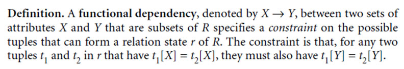
1. Functional Dependencies

• Normal forms: a set of rules to avoid redundancy and inconsistency.
• Require the concepts of
  • functional dependency (FD, most important: up to BCNF)
  • multivalued dependency (MVD for 4NF)
  • join dependency (5NF)
• Seven Common Normal Forms in ascending order: 1NF, 2NF, 3NF, BCNF, 4NF, 5NF, DKNF.
• Higher normal forms are more restrictive.
• A relation is in a higher normal form implies that it is in a lower normal form, but not vice versa.

Example:

If a relation is in BCNF, then it is also in 3NF, 2NF and 1NF.

If a relation is in 2NF, then

1. It is in 1NF,
2. it may or may not be in 3NF, and
3. it may or may not in BCNF.

If a relations is not in 3NF, then

1. It is not in BCNF.
2. It may or may not be in 1NF or 2NF.

• In general, the higher the normal forms a relation is in, the better the design of the relation in terms of avoiding redundancy and inconsistency.
• However, it may be necessary to consider other issues, especially performances.
  • Higher normal forms may be achieved by decomposition, resulting in more relations. More joins may thus be needed to provide the data for a query.
• 1NF and 2NF are more interesting for historical reasons.
• 4NF and 5NF involves the concept of multivalued and join dependencies (MVD and JD). They are hard to understand and even harder to use in most situations.
• Domain Key Normal Form (DKNF) involves the concept of constraints.
• Based on the concept of functional dependencies (FD), the most important normal forms are
  • 3NF and
  • BCNF (Boyce-Codd Normal Form).

Functional Dependencies (FD):

• Types of relationship between attributes:
  • Many to one (0..* to 0..1)
  • Many to many (0..* to 0..*)

Example

Many to many relationships.

Consider the relation Enrol:

Under reasonable assumptions, there are many to many relationships between the attributes

1. Course and Student: course may enrol many students; a student may take many courses)
2. Course and Grade
3. Student and Grade
4. {Course, Grade} and Student: both S2 and S3 have a grade of B in Course C1.

However, the relationship between {Course, Student} and Grade is not a many-to-many relationship if we assume that a student can only has one grade for a given course.

• A many to many relationship between two attributes means that there is no constraint and no dependency between the values of the attributes.

Example

Many to one relationships.

For many applications, the relationship between SS# and NAME are many to one.

SS#        ->     NAME
(many)            (one)

Interpretations and terminology:

1. Many different SS#'s (persons) may have the same NAME.
2. Given a SS#, there can only be one NAME associated with it (not allowing alias, etc).
3. There should not be two tuples with the same SS#, but different NAME. 
4. SS# uniquely determines NAME.
5. NAME is functionally determined by SS#.
6. There is a functional dependency SS# --> NAME.
7. Hence, a functional dependency specifies a many to one relationship between attributes.

For example,

is not allowed if we assume SS# -> NAME.

Example

In a university, there may be a many-to-one relationship between {COURSE#, STUDENT#} and GRADE.

Interpretations:

1. A student may have only one grade for a course.
2. We say  there is a functional dependency:
   • COURSE# STUDENT# --> GRADE
   • {COURSE#, STUDENT#} determines GRADE.
3. Note that under different assumptions, the functional dependency may not be true.
4. For example, if a student is allowed to retake a course, then he may have two grades for the same course (in different semesters), then COURSE# STUDENT# --> GRADE  is false.
5. We may actually have COURSE# STUDENT# SEMESTER --> GRADE

• Hence, functional dependency is a result of the requirements and business logics of the applications. 
• There is no universally true non-trivial functional dependency.
• In other words, functional dependencies depend on the semantic of the problems.

Example

In most application, we have

SS# --> NAME             (i.e.  a person has only one SS#.)

However, in a criminal database, several bad guys may use the same fake SS#, and thus

SS# --> NAME  is not true.

Or, if you are dealing with an international data base with many countries.  Each country may has its own SS#.  Two countries may issue the same SS#.  Hence,

SS# --> NAME   is not true.

We may instead have  SS# COUNTRY --> NAME.

• A relation scheme R is said to satisfy the functional dependency X --> Y if for any relation r that uses R, if there are two tuples s and t in r such that s[X] = t[X], then s[Y] = t[Y].
• i.e.  the same value of X implies the same value of Y.
• Definition of FD from EN:

Example

SS# --> SNAME:

There are no two tuples with the same SS# but different names.

DEPT-NO --> MANAGER-NO:

There are no two tuples with the same DEPT-NO but different MANAGER-NO.  A department has only one manager.

SUPPLIER# PNUM DATE --> QUANTITY

There are no two tuples with the same SUPPLIER#, PNUM and DATE but different QUANTITY.  That is, any supplier has only one shipment of a part on a given date.

Armstrong's axioms

• A set of axioms for inference with FD: http://en.wikipedia.org/wiki/Armstrong%27s_axioms.
• Axioms: 'self-evidence' or 'assumed'.
• Three basic axioms:
  1. Reflexivity: If X and Y are sets of attributes and Y is a subset of X, then X --> Y.
  2. Augmentation: If X --> Y then X Z --> Y Z.
  3. Transitivity: If X --> Y and Y --> Z then X --> Z
• Three additional rules that can be proven by the basic axioms.
1. Pseudo-transivitiy Rule: If X--> Y, YZ -> A then XZ -> A
2. Decomposition Rule: If X --> Y Z, then X --> Y and X --> Z.
3. Union Rule:  If X --> Y and X --> Z then X --> Y Z.
• Armstrong's axioms are sound and complete.
  • Sound: implies only FD that are correct.
  • Complete: can be used to imply all correct FD.
• CS students need to know how to infer using a formal mathematical model.

Example

Let X be CITY STREET, Y be STREET, then Y is a subset of X, and X --> Y or CITY STREET --> STREET. (Reflexivity).

• If two tuples have the same value of CITY STREET, then they have the same value of STREET.
• This is so trivial that we call a functional dependency likes CITY STREET --> STREET a trivial functional dependency. They do not actually specify a business requirement

A --> A and B C --> B are trivial.

• Since trivial functional dependencies do not actually give you any information, we are only interested in non-trivial functional dependency.

If EMP-NO  -->  DEPT-NO and DEPT-NO  -->  MANAGER-NO
then EMP-NO  -->  MANAGER-NO.

Interpretation: If

• every employee works for only one department, and
• every department has only one manager, then

then every employee has only one manager.

Example

Prove the union Rule.

Proof.

(1) X -> Z (given)
(2) X X -> X Z (augmentation of (1) with X)
(3) X -> XZ (simplification of (2))
(4) X -> Y (given)
(5) XZ -> YZ (augmentation of (4) with Z)
(6) X -> YZ (transitivity on (3) and (5))

Exercise

Prove the pseudo transitivity rule.

Keys and Superkeys

• We can use functional dependencies to define keys and superkeys.
• For a relation scheme R, K is a candidate key if
  • Uniqueness:  K --> R.
  • Minimality:  there is no proper subset of K that determines R.
• K is a superkey if K --> R.

Example

In EMPLOYEE(EMP-NO, DEPT-NO, MANAGER-NO) with

EMP-NO --> DEPT-NO and
DEPT-NO --> MANAGER-NO.

By the transitivity axiom, EMP-NO --> MANAGER-NO.
By the union rule, EMP-NO --> EMP-NO DEPT-NO MANAGER-NO.
                       
Hence, EMP-NO is a key of EMPLOYEE(EMP-NO, DEPT-NO, MANAGER-NO).

On the other hand, DEPT-NO is not a key since we do not have DEPT-NO --> EMP-NO.

Furthermore, there are four superkeys:

1. EMP-NO
2. EMP-NO, DEPT-NO
3. EMP-ND, EPT-NO, MANAGER-NO

Closure of Attributes

• Given a set of FD F, the closure of a set of attributes X, denoted as X+, is the set of all attributes functionally determined by X using Armstrong's axioms on F.

Example

Cons der:

F = {A-> B, BC -> DA, BD -> C, E-> A, AC -> DE }

We have

A+ = AB
B+ = B
C+ = C
D+ = D
E+ = E
(AB)+ = AB
(AC)+ = ABCDE
(AD+ = ABCDE
(AE)+ = ABE
(BC)+ = ABCDE
(BD)+ = ABCDE
(BE)+ = ABE
(CD)+ = CD
(CE)+ = ABCDE
(DE)+ = ABCDE
(ABC)+ = ABCDE
...
(ABE)+ = ABE
...

• There are thus six candidate keys: AC, AD, BC, BD, CE and DE.
• This is a theoretical example not likely to appear in the real world, especially if you conduct a good data modeling.
• The closure of attributes can be used for other purposes, such as checking validity of FD, computing closure of a set of functional dependencies, checking equivalence of two set of FDs, etc.

Algorithm for finding X+ for a set of FDs F.

X+ <- X
while (there exists a FD P -> Q such that P is a subset of X+ and there are attributes K in Q that is not in X+) {
   X+ <- X+ U Q
}

Closure of a set of functional dependencies

• The closure of a set of FD, F, is denoted by F+ and is the set of all FDs that are logically implied by F.

Example

Consider F = { A->B, B->C }

F+ = {
A->A, A->B, A->C, A-> AB, A-> AC, A-> BC, A->ABC,
B->B, B->C, B->BC,
C->C,
AB->A, AB->B, AB->C, AB->AB, AB->AC, AB->BC, AB->ABC,
AC->A, AC->B, AC->C, AC->AB, AC->AB, AC->BC, AC-> ABC,
BC->B, BC->C, BC->BC,
ABC->A, ABC->B, ABC->C, ABC-> AB, ABC-> AC, ABC-> BC, ABC->ABC }

Note that

• Some FD in F+ are trivial. Trivial FDs, such as A->{} may also be included.
• FD+ itself is not very interesting.

Equivalence and cover

• Two sets of FD, F and G are equivalent, if F+ = G+. They are covers of each other.
• The attribute A in the FD P-> Q is extraneous for a set of FDs F if F - {P-> Q} U {P-A -> Q} is equivalent to F.

Example

Consider the F = { A->B, AB->C }.

B is extraneous since for G = { A->B, A->C }, F+ = G+.

• A FD f in F is redundant if (F - f)+ = F.

Example

In F = {A->B, AB->C, B->C },

A->C is redundant.

• A canonical cover, G, of F satisfies the following conditions:
  • G is a cover of F; G+ = F+.
  • There is no redundant FD in G.
  • There is no extraneus attribute in G.
  • The left hand side of every FD in G is unique.
• A minimal cover, G, of F satisfies the following conditions:
  • G is a cover of F; G+ = F+.
  • There is no redundant FD in G.
  • There is no extraneus attribue in G.
  • The right hand side of every FD in G contains only a single attribute

In F = {A->B, AB->C, B->C, A->D},

G1 = {A->B, B->C,A->D} is a minimal cover.

G2 = {A->BD, B->C} is a canonical cover.

• The minimal covers and canonical covers are simplified versions of a set of FDs,
• They are useful in understanding the FD and for proper decompositions to resolve unnecessary redundancy.

Exercise:

Consider F: {A->C, BCD->A, C->E, CD-> A, AB->C }

1. Does F imply BD-> A (i.e. F |= BD -> A)?
2. F |= AE -> B ?
3. Give a canonical cover for F?
4. Show all candidate keys.

Exercise:

Consider F: {AB->CE, BC->D, D->BC, C->E, A->C, A->E}

Find:

• all candidate keys.
• a canonical cover of F.

Exercise:

Can there be more than one canonical covers for a set of FDs?

2. Normal Forms using Functional Dependencies

First Normal Form

• A relation is in 1NF if all attribute values are atomic: no repeating group, no composite attributes.
• Formally, a relation may only has atomic attributes.  Thus, all relations satisfy 1NF.

Example

Example:   Consider the following table.  It is not in 1 NF.

The corresponding relation in 1 NF:

• Why atomic: relational theory and operations treat attributes as atomic.
• Relations satisfying only 1NF has unnecessary redundancy and anomalies.

Example

Consider the tuple (Empid: 12345, OSSkills: "Windows, Linux, Solaris").

• It will be difficult to identify all employees with Linux skills.
• Data entry problems and issues, e.g. Linux linux, linx, etc., may further degrade data qualtiy and introduce inconsistency.

Second Normal Form

• A relation R is in 2NF if
  • R is in 1NF, and
  • all non-prime attributes are fully dependent on the candidate keys.
• A prime attribute appears in a candidate key. Otherwise, it is a non-prime attribute.
• There is no partial dependency in 2NF.
• If X -> A, A is a non-prime attribute, and X is a subset of a candidate key K, then X = K.

Example

The following relation is not in 2NF.  (Assume the number of credits of a given course does not change).  Note the redundancy and anomalies.

That is, we assume:

• Course -> Credit
• Course, Student -> Grade

Thus,

1. Course, Student is the only candidate key.
2. Prime attributes: Course, Student
3. Non-prime attribute: Credit, Grade.
4. (1) is a violation of 2NF.

Third Normal Form

• (Old definition) A relation R is in 3NF if
  1. R is in 2NF, and
  2. There is no transitive dependency of nonkey attributes on the keys.

Example

• The following relation may be in 2NF, but may not be in 3NF.

• If we assume:
  • EMP_NO -> NAME, DEPT_NO
  • DEPT_ NO -> MANAGER_NO
• then
  • there is one candidate key: EMP_NO
  • Prime attributes: EMP_NO
  • Non-prime attributes: NAME, DEPT_NO, MANAGER_NO.
  • The relation is in 2NF.
  • The relation is not in 3NF because of the transitive FD: EMP_NO -> MANAGER_NO via the non-prime attribute DEPT_NO.

Example

Consider the relation

S(SNUM, PNUM, SNAME, QUANTITY) with the following assumptions:

1. SNUM is unique for every supplier.
2. SNAME is unique for every supplier.
3. QUANTITY is the accumulated quantities of a part supplied by a supplier.
4. A supplier can supply more than one part.
5. A part can be supplied by more than one supplier.

We have the following non-trivial functional dependencies:

1. SNUM --> SNAME
2. SNAME --> SNUM
3. SNUM PNUM --> QUANTITY
4. SNAME PNUM --> QUANTITY

Note that SNUM and SNAME are equivalent.

The candidate keys are:

1. SNUM PNUM
2. SNAME PNUM

Prime attributes: SNUM, PNUM, SNAME

Non-prime attribute: QUANTITY.

The relation is in 3NF.

Example

Consider the relation R(CITY, STREET, ZIP) with the FDs:

1. CITY STREET --> ZIP, and
2. ZIP --> CITY.

There are two candidate keys:

1. CITY STREET, and
2. ZIP STREET

Hence, all attributes are prime attributes and the relation is in both 2NF and 3NF.

Note that a relation such as EMPLOYEE(EMP_ID, EMP_NAME, Street, City, Zip, State) is not in 3NF.

This is a classical example you can find in many database textbook. The FDs may not be correct in the United States. See, for example: Why all 5-digit ZIP Code™ lists are obsolete.

• 3NF does not eliminate all redundancy due to functional dependencies.

BCNF (Boyce-Codd Normal Form)

• A relation R is said to be in BCNF if for every non-trivial functional dependency X --> A in R, X is a superkey.

Example                  

EMPLOYEE(EMP_NO, NAME, DEPT_NO, MANAGER_NO) with

EMP_NO --> NAME
EMP_NO --> DEPT_NO
DEPT_NO --> MANAGER_NO

is not in BCNF.

The functional dependency  DEPT_NO --> MANAGER_NO is

(1)  non-trivial, and
(2)  DEPT_NO is not a superkey.

• Recall that this is the example we used for illustrating bad design.
• This is also not in 3NF.

We can decompose

EMPLOYEE(EMP_NO, NAME, DEPT_NO, MANAGER_NO) into

EMP(EMP_NO, NAME, DEPT_NO) with

EMP_NO --> NAME
EMP_NO --> DEPT

and

DEPARTMENT(DEPT_NO, MANAGER_NO) with

DEPT_NO --> MANAGER_NO

Both relations are in BCNF since

• EMP_NO is a superkey of the relation EMP.
• DEPT_NO is a superkey of the relation DEPARTMENT.

Recall that these are the good relations without the anomalies in the previous example.

Example    

Consider the relation

S(SNUM, PNUM, SNAME, QUANTITY) with the following non-trivial functional dependencies:

1. SNUM --> SNAME
2. SNAME --> SNUM
3. SNUM PNUM --> QUANTITY
4. SNAME PNUM --> QUANTITY

Note that SNUM and SNAME are equivalent.

The candidate keys are:

1. SNUM PNUM
2. SNAME PNUM

Prime attributes: SNUM, PNUM, SNAME

Non-prime attribute: QUANTITY.

S is not in BCNF because, for example, the functional dependency 

SUPP# --> SNAME is

• non-trivial, and
• SNUM is not a superkey.

To deal with it, we can decompose S(SUPP#, PART#, SNAME, QUANTITY) into

(1) SUPPLIER(SNUM, SNAME) with  

SNUM --> SNAME
SNAME --> SNUM

with two candidate keys:

1. SNUM
2. SNAME

(2) ORDER(SUPP#, PART#, QUANTITY)  with 

SNUM, PNUM --> QUANTITY.

Example 4:  Consider the relation R(A, B, C, D) with

A --> B,  B --> C, C --> A and C --> D.

There are three candidate keys:

• A
• B, 
• C.

Since every left hand side of any non-trivial functional dependency is a superkey,  R is in BCNF.

Motivation of BCNF

• The purpose of BCNF is to eliminate any redundancy that functional dependencies can made.
  • In a BCNF relation, no value can be predicted from any other attributes, using only functional dependencies.
  • This is because in a BCNF relation, using functional dependencies only,
    • any value can only be determined by a superkey,
    • but the superkey is unique.
  • However, there are other type of dependencies.
  • Therefore, there are higher normal forms.

Consider the relation R(CITY, ZIP, STREET)
       
Using the code for the postal office, we have

CITY STREET --> ZIP, and ZIP --> CITY.

Hence, there are two candidate keys:

1. CITY STREET, and
2. ZIP STREET

Therefore, R is not in BCNF since in ZIP --> CITY, ZIP is not a superkey.

However, if we decompose R into two relations, each with two attributes, then the functional dependency

CITY STREET --> ZIP is lost

Therefore, we better leave the relation alone.

• Sometimes it is not possible for a relation to be in BCNF ==> need a less strict normal form (3NF).

Third Normal Form Revisited

• The new definition of 3NF: a relation R is said to be in the third normal form if for every non-trivial functional dependency X --> A,
  • X is a superkey, or
  • A is a prime (key) attribute.
• 3NF cannot eliminate all redundancy due to functional dependencies.

Example 

For the relation R(CITY, ZIP, STREET)
       
Using the code for the postal office, we have

CITY STREET --> ZIP, and ZIP --> CITY.

Hence, there are two candidate keys:

1. CITY STREET, and
2. ZIP STREET

Hence,

Prime attributes: STREET, CITY, ZIP

R is in the 3NF because

• For the non-trivial FD CITY STREET --> ZIP, CITY STREET is a superkey.
• For the non-trivial FD ZIP --> CITY, CITY is a prime attribute.

Example 

Reconsider the relation

S(SNUM, PNUM, SNAME, QUANTITY) with the following non-trivial functional dependencies:

1. SNUM --> SNAME
2. SNAME --> SNUM
3. SNUM PNUM --> QUANTITY
4. SNAME PNUM --> QUANTITY

Note that SNUM and SNAME are equivalent.

The candidate keys are:

1. SNUM PNUM
2. SNAME PNUM

Prime attributes: SNUM, PNUM, SNAME

Non-prime attribute: QUANTITY.

S is in 3NF because

• For the non-trivial FDs (1) and (2), the right hand sides are prime attributes (SNAME and SNUM).
• For the functional dependencies (3) and (4), the left hand sides are superkeys.

Example 

Reconsider

EMPLOYEE(EMP_NO, NAME, DEPT_NO, MANAGER_NO) with

EMP_NO --> NAME
EMP_NO --> DEPT_NO
DEPT_NO --> MANAGER_NO

is not in 3NF.

The functional dependency  DEPT_NO --> MANAGER_NO is

(1) non-trivial,
(2) DEPT_NO is not a superkey, and
(3) MANAGER_NO is not a prime attribute.

Normalization Theory Using Functional Dependencies

• To use the theory on functional dependency:
  • For a relation of a set of attributes, we analyze the assumptions of the applications.
  • From the assumptions, we obtain the functional dependencies.
  • We determine the candidate keys and prime attributes.
  • If the relation is not in BCNF, we perform decomposition.
  • If BCNF cannot be satisfied, we aim for 3NF.

3. Decomposition

• Decomposition is a major tool for generating relations satisfying normal forms.
• Decomposition should be disciplined:
  • More relations may be less efficient in storage.
  • More relations may be less efficient in executing query.
  • Some decompositions are harmful:
    • Lossy decompositions.
    • Decompositions that do not preserve dependencies.
• Hence, it is important to have lossless dependency-preserving decomposition.

Lossy Decomposition

Example:

Consider the relation EMP(EMP_NO, DEPT, MGR_NO) with 

EMP_NO -->  DEPT
DEPT -->  MGR_NO

Note that we do not have MGR_NO --> DEPT, since one manager can manage more than one departments under the assumptions made for this example.

          
The relation is not in BCNF because of the FD

DEPT --> MGR_NO

Suppose we decompose the relation into

EMP1(EMP_NO, MGR_NO)
DEPT(DEPT, MGR_NO)

They are obtained by projections from EMP:

EMP1:                     

DEPT:

If we do not loss any information by the decomposition, we should get the original relation from the natural join.

However,  EMP1 |x| DEPT is     

         
This is not the same as the original relation EMP. Spurious tuples were incorrectly created.

Hence, the decomposition of EMP(EMP_NO, DEPT, MGR_NO) into
 
EMP1(EMP_NO, MGR_NO) and
DEPT(DEPT, MGR_NO)

is lossy.  It is not a good decomposition.

Lossless Decomposition

Example:

Consider now the following decomposition of EMP(EMP_NO, DEPT, MGR_NO):

EMP2(EMP_NO, DEPT)  and
EMP3(EMP_NO, MGR_NO)

We have EMP2 and EMP3:

EMP2:                     

EMP3:

Hence, EMP2 |x| EMP3:

This is exactly the same as the original relation EMP.  Therefore, the decomposition does not loss any information.  It is a lossless decomposition.

Theory of Lossless Decomposition

Example:

Why is the decomposition of EMP(EMP_NO, DEPT, MGR_NO) into

(1) EMP1(EMP_NO, MGR_NO) and DEPT(DEPT, MGR_NO) lossy, and

(2) EMP2(EMP_NO, DEPT) and EMP3(EMP_NO, MGR_NO) lossless?

Theorem: Suppose R(X, Y, Z) is decomposed into R1(X, Y) and R2(X, Z).  X is the set of common attributes in R1 and R2.  The decomposition is lossless if and only if

(a) X --> Y, or
(b) X --> Z.

Example:

In case (1), X is MGR_NO, Y is EMP_NO, Z is DEPT.

None of condition (a) or (b) is satisfied.  Hence, (1) is lossy.

In case (2), X is EMP_NO, Y is DEPT, Z is MGR_NO.

Both conditions (a) and (b) are satisfied.  Hence, (2) is lossless.

• For decompositions into more than two relations, use the chase matrix algorithm (EN Algorithm 16.3).

Example:

Consider R(A,B,C,D,E) with {A->BC, CD -> E, BA -> C, D->B}.

It is decomposed into R1(A,B), R2(A,C), R3(C,D,E) and R3(B,D).

Step 1. Create a table of 5 columns (number of columns and 4 rows (number of relations). Populate it with b(i,j).

Step 2. For each relation Ri, set all attribute Aj that appears in Ri from b(i,j) to a(j).

Step 3. For each FD X-> Y, with two rows have the common X values, for every attribute W in Y:

• If one cell is an a and the other cell is an b, change the b to the a.
• If both cells are b's, change them to the same b.

Applying A-> BC:

Applying CD -> E: no change since no row has the same values in CD.

Applying BA -> C: no change since R1 and R2 already have the same a's value: A(3).

Applying D->B

Since there is no row with only a's, the decomposition is lossy.

Example:

Now suppose that C->DE is also in the FDs. That is, we have:

R(A,B,C,D,E) with {A->BC, CD -> E, BA -> C, D->B, C->DE}.

We will have one more step.

Applying C->DE:

Now we have two rows with only a's and thus the decomposition is lossless.

Dependency-Preserving Decomposition

Example:                        

For the relation EMP(EMP_NO,DEPT,MGR_NO) with 

EMP_NO -->  DEPT
DEPT -->  MGR_NO,

The decomposition of EMP into

EMP2(EMP_NO, DEPT)  and
EMP3(EMP_NO, MGR_NO)

is lossless, but it does not preserve dependencies:

the FD  DEPT --> MGR_NO

cannot be enforced by any relation after the decomposition.

For example, if we add the information EMP 23000 work in the ACCT department under manager 97000 and are not careful, we may have:

 EMP2:                     

EMP3:

The FD  DEPT -->  MGR_NO is violated.

Thus, for the relation EMP(EMP_NO,DEPT,MGR_NO) with 

EMP_NO -->  DEPT
DEPT -->  MGR_NO,

the best decomposition is into

EMP1(EMP_NO, DEPT)  and
DEPT(DEPT, MGR_NO)

It is easy to show that, the decomposition is lossless, preserves dependencies, and that EMP1 and DEPT are both in BCNF.

• It is possible to decompose a relation such that
  • all member relations are in 3NF,
  • the decomposition is lossless, and
  • all FDs are preserved.
• It is possible to decompose a relation such that
  • all member relations are in BCNF, and
  • the decomposition is lossless, but
  • all FDs may not be preserved.

Algorithm for decomposition in 3NF relations

• See Algorithm 16.6 of EN: lossless FD preserving decomposition into relations in 3NF.

Example:

Consider R(A,B,C,D,E) with F = {A->BC, CD -> E, BA -> C, D->B}.

Step 1 Find a canonical cover (as opposed to a minimal cover in EN) G for F.

The FD BA->C is redundant.

G = {A->BC, CD -> E, D->B}.

Step 2. For every FD X->Y in G, create a relation with the schema XY and add it to the result D.

Relations created:

R1(A,B,C) with A->BC
R2(C,D,E) with CD->E
R3(B,D) with D->B

It can be seen very easily that R1, R2 and R3 are all in 3NF. Furthermore, all FDs are preserved.

Step 3. If no relation in D contains the key of R, create a new relation with the key of R being the schema and add it to the result D.

There is only one candidate key of R: AD. Since none of R1, R2 and R3 contains A, create the relation

R4(A,D) with no FD

Step 4. Simplify D by removing relations that are redundant (i.e. that its schema is a subset of the schema of another relation).

No action as there is no redundant relation.

Example:

Consider R(A,B,C,D) with {A->BC, BC->D, D->C}

Using the algorithm, the result of decomposition contains two relations:

R1(A,B,C) with {A-> BC} and
R2(B,C,D) with {BC->D, D>C}

R3(C,D) is removed as redundant in the last step of the algorithm.

R1 and R2 are both in 3NF but R2 is not in BCNF.

• Algorithm 16.5 of EN is an algorithm for lossless decomposition into BCNF but FD may not be preserved.
• Sometimes, it is not possible to decompose a relation into two relations losslessly and preserve all FD, just to achieve BCNF.

Example:

Consider the relation R(A, B, C) with A -> B and C -> B.

R is not in 2NF.  It is not possible to decompose R into two relations losslessly while preserving all functional dependencies.

However, it is possible to decompose into three relations losslessly and with all functional dependencies preserved:

R1(A, B),
R2(B, C) and
R3(A, C).

4. Higher Normal Forms

Multivalued Dependencies

• BCNF guarantees that there is no anomaly related to functional dependencies.  However, there are other forms of redundancy.

Example 1:

Consider the following instance of the relation R(Emp_No, Dept, Skill):

There are no non-trivial functional dependencies.  R is in BCNF.

If the department an employee is working on is independent of the skill that he has, there is redundancy. For example, the fact that employee 100 has the skill PHP is stored twice.

• Let A, B, C be the three distinct sets of attributes in R(A,B,C).  There is a multivalued dependency (MVD) of B on A, A ->-> B, if the set of B values associated with a given A value is independent of the value of C.  A is said to multidetermine B.

Example 2:

Under the assumption of the previous example, we have

Emp_No ->-> Dept and
Emp_No ->-> Skill.

Suppose we have the following relation instance under a different set of assumptions:

Without knowing the underlying assumptions, this instance of the relation implies that the multivalued dependency Emp_No ->-> Dept does not hold true since

• for a given Emp_No (e.g. 100), skill is not independent of Dept. 
  • When Dept is D101, skills are {PHP, MySQL} and
  • when Dept is D102, skills are {PHP}.

Note:

• An instance of a relation cannot be used to prove that a FD is valid for a relation schema (since a FD is the result of application require mens and must be held for every instance, not just one.)
• An instance of relation may be used to prove that a FD is not valid for a relation schema: by providing two tuples that violate the FD.

A more precise definition of MVD: 

• Let A, B, C be the three distinct sets of attributes in  R(A,B,C).  A ->-> B is true iff the following condition is true.  For every two tuples t1 and t2 in R such that t1(A) = t2(A), then there exist t3 and t4 in R such that t3(A) = t4(A) = t1(A), t3(B) = t1(B), t4(B) = t2(B), t3(C) = t2(C) and t4(C) = t1(C).

Example 3:

Consider Example 1 again. In the data modeling, there may be two classes with a many-to-many association.

• Employee: with key EMP_NO and a multi-valued attribute SKILL.
• Department: with key DEPT

If one follows the data modeling and the mapping to relation guideline, two relations will be created (instead of one).

This shows the importance of good data modeling.

• Intuitive explanation: If in R(X,Y,Z), X->->Y and X->->Z, then there are independent many-to-many relationships between X and Y, and X and Z.

Some Properties Of Multivalued Dependencies

• For R(A,B,C), A ->-> B => A ->-> C.
• If A -> B, then A ->-> B.
• A ->-> B and V is a subset of W => AW ->-> VB
• Note that, in general, X ->-> Y and Y ->-> Z do not imply that X ->-> Z.

Fourth Normal Form

• A relation R is in the fourth normal form (4NF) if
  • (1) R is in BCNF and
  • (2) all MVD are either trivial or can be derived from a FD.
• 4NF => BCNF.
• A relation in 4NF does not have redundancy due to FD or MVD.

Example 4:

The relation R(Emp_No, Dept, Skill) in Example 1 is in BCNF but not in 4NF.  It should be decomposed into:

R1(Emp_No, Dept) and
R2(Emp_No, Skill).

Note that these two relations are created with good data modeling and mapping to relations.

• Decomposition to overcome 4NF: if R(A,B,C) is in BCNF and A ->-> B, then decompose the relation into
  • R1(A,B) and
  • R2(A,C).

Embedded Multivalued Dependencies

• FD and MVD are not the only form of data dependency.

Example 5:

Consider the following relation R(Proj_No, Emp_No, Skill):

For this application, each project (Proj_No) has a number of employees (Emp_No) and each project requires a list of skills (Skill).  We have:

Proj ->-> Emp_No
Proj ->-> Skill.

An employee provides some skills that a project needs.  If an employee has a skill that is not needed by the project (e.g. employee E1 may have the skill of 'Internet'), the skill is not stored in the tuples of project P1, which does not require the skill 'Internet'.

Note that Emp_No ->-> Skill does not hold in R.

R is not in 4NF.

We can decompose the relation into two relations:

R1(Proj_No, Emp_No) and
R2(Proj_No, Skill)

R1:                        

R2:

Both R1 and R2 are now in 4NF.

However, if skill is a multi-valued attribute of an employee, then we should have

Emp_No ->-> Skill

It does not show up in R because it is embedded. If we project R to remove PROJ_NO, this relationship appears.

These embedded MVD's are not enforced by the relations R1 and R2.

These MVD's only display themselves after projection.

We may have the following three classes with three many-to-many associations between each pair of them:

• Project: with key PROJ_NO
• Employee: with key EMP_NO
• Skill: with key SKILL

Decomposition of R into R1 and R2 will lose this embedded multivalued dependency. 

• Let X, Y and Z be subsets of attributes of the relation scheme r.  A relation R over the scheme r satisfies the embedded multivalued dependency X ->-> Y | Z if X ->-> Y in the relation π(X U Y U Z)(R).  X, Y and Z need not be disjoint.

Example 6:

There are (trivial) embedded MVD's Emp_No ->-> Skill | φ and Emp_No ->-> Proj_No | φ in R of the previous example.

To remedy the problem, decompose the relation R into:

R1(Proj_No, Emp_No)
R2(Proj_No, Skill) and
R3(Emp_No, Skill).

All relations are in 4NF (5NF too) and the embedded MVD are not lost.

• The previous examples show that it may not be possible to decompose a relation R into two relations and preserve all dependencies but it may be possible to decompose R into more than two relations and preserve all dependencies.
• Note that there is no embedded FD, only embedded MVD.

Example 7:

Consider an application with four classes A, B, C and D with primary keys A_ID, B_ID, C_ID and D_ID.  There are many to many binary associations between A and C as well as B and C.  Furthermore, there is a ternary association between A, B and D.

If somebody has not performed a good data modelling, it is possible to come up with a relation R(A_ID, B_ID, C_ID, D_ID).

However, the MVD C_ID ->-> A_ID (or C_ID ->-> B_ID) is not true in R because of the additional attribute DID.  If the attribute D_ID is removed by projection, then the independence between A_ID and B_ID for a given value of C_ID will show up.  Hence, there is a embedded MVD C_ID ->-> A_ID | B_ID in R.

Join Dependencies

• Given a relation scheme r and a projection {R1, R2, ..., Rn} of r.  A relation R on r satisfies the join dependency (JD) *[R1, R2, ..., Rn] iff πR1(R) |x| πR2(R) ... |x| πRn(R) = R.
• In other word, there is a lossless decomposition of R into R1, R2, ..., Rn.
• A JD is trivial if one of Ri is R.

Example 8:

In Example 5 with embedded MVD, there is a non-trivial JD of R(Proj_No, Emp_No, Skill):

{{Proj_No, Emp_No}, {Proj_No, Skill}, {Emp_No, Skill}}

Fifth (Project-Join) Normal Form

• A relation R satisfies the fifth normal form (5NF) or Project-Join Normal Form (PJNF) if for every non-trivial join dependency *[R1, R2, ..., Rn] of R, Ri is a superkey of the original relation.
  

Example 9:

The relation R(Proj_No, Emp_No, Skill) of Example 3 does not satisfy 5NF.

• 5NF => 4NF but not the other way around.

Domain-Key Normal Form

• Domain Constraint (DC), In(Ai, Di): if the value of the attribute Ai of the relation R must be in the domain Di.
• Key Constraint (KC):  KEY(K): for the key K of a relation R, no two tuples of the relation R has the same K value.
• General Constraint (GC): A general constraint is a predicate statement such that every tuple in the relation must satisfy the GC in order for the tuple to be valid.
• A relation is in domain key normal form (DKNF) if all its GC's are natural consequence of its DC and KC.

Example 10:

Consider the relation scheme Enrolment(Course_No, Student_No, Grade)

The key is {Course_No, Student_No}.

KC: Course_No, Student_No -> Grade.

DC:

Domain(Course_No): 001..999 (i.e. In(Course_No, {001..999}
Domain(Grade): {A,B,C,D,F,I,P}
Domain(Student_No): string(1..10)

GC:

One of the GC may be:

if Course_No mod 10 >= 8 then
   (Grade ε {'P', 'F', 'I'}
else
   (Grade ε {'A', 'B', 'C', 'D', 'F', 'I'};
end if;

The relation Enrolment is in PJNF.

However, the relation Enrolment is not in DKNF since the GC is not a natural consequence of the KC and DC.

To solve the problem, we may make the following decomposition:

Pass_Fail_Course_Enrolment(Course_No, Student_No, Grade) with

DC: 

Domain(Course_No): {I | I ε 1..999 and I mod 10 >= 8}
Domain(Grade): {'F', 'I', 'P'}

Regular_Course_Enrolment(Course_No, Student_No, Grade) with

DC:              

Domain(Course_No): {I | I ε 1..999 and I mod 10 < 8}
Domain(Grade): {'A', 'B', 'C', 'D', 'F', 'I'}

Both relations are now in DKNF. However, this is usually not done. Instead, stored procedures may be used to enforce the constraint.

Example 11:

A non-trivial FD is a GC.
A FD with the determinant being a key is a KC.

Hence, if a relation satisfies BCNF, then all its FD can be deducted from KC.

If a relation does not satisfy BCNF, then there is a FD with a non-key determinant.  Thus, it will not satisfy DKNF too.

Example 12:                    

A non-trivial MVD is a GC.
There is no way to express a MVD using KC or DC.

Thus, if a relation is not in 4NF, it is also not in DKNF.

• In fact, DKNF => PJNF but not vice versa.
• DKNF is the highest normal form.
• There exists no simple algorithm that helps in the design of DKNF.
• It is unlikely that applications with complex constraints can be converted to DKNF.
• It is also difficult to infer using MVD, embedded MVD or JD.
• Thus, BCNF and 3NF are usually the highest normal forms for many practical applications.